Methodology
1. Calculation using Origin-Destination Matrix (OD-Matrix)
First we extract MasterPlan 14 Subzone (no sea) and export it into a GeoPackage. We also add in the education layer, after filtering Junior Colleges, Mixed Levels and Institutions, using the ‘filter by expression’ function into QGIS and export this layer to GeoPackage.
The roads layer from the OSM data is also added onto the panel. The roads layer is then clipped together with MasterPlan 14, to get roads that are within Singapore. This newly created clipped layer is then exported as GeoPackage.
A hexagon layer, with the shape of MasterPlan 14 is also created using the ‘Create Grids’ function. The hexagon is then computed as a hexagon centroid so as to ‘convert’ the polygon feature into a point feature which could then be runned by QNEAT3 for network analysis.
After using QNEAT3 for accessibility analysis, we would obtain an Output OD Matrix which shows the shortest path which is then categorised by a choropleth map.
2. Calculation on number of nearest bus stops, LRT and MRT station within 1km buffer region
A dissolved buffer region of 1 km with locations of Junior Colleges being the centre of the buffer region, using the ‘buffer’ function and exported as GeoPackage.
For bus stops, we would use the transport layer under OSM data, clip to filter transports within Singapore and further filter for bus stops. Lastly, to filter those bus stops within the 1 km buffer region.
Clip the LRT and MRT Exit (downloaded from data.gov) layer with the 1 km buffer region to get MRT and LRT stations within the 1 km buffer region.
Step-By-Step Guide
2.1 Data Collection and Preparation
2.1.1 Downloading Geospatial Data
Download the following geospatial data from data.gov.sg:
- Master Plan 2014 Subzone Boundary (No Sea)
Download School Directory and Information from data.gov.sg
- Extract general-information-of-schools.csv from the zip file downloaded
Download GIS data from OpenStreetMap (OSM)
- malaysia-singapore-brunei-latest-free.shp.zip
Download the following data from data.gov.sg
- Lta-mrt-station-exit
2.1.2 Managing the Imported Data
Create a new project folder called “Subtheme1” and create a new sub-folder called data.gov
Unzip the newly downloaded data and place them into the sub-folder
Create another sub-folder called GeoPackage
- Within GeoPackage, create another sub-folder called SG
2.2 Setting the Scene
2.2.1 Starting a new QGIS project
Launch QGIS
Start a new QGIS project
Save the project in Subtheme1 folder and name the new project as Subtheme1
Ensure that the CRS is in SVY21/EPSG3414 at the lower right corner of the QGIS software
2.2.2 Preparing the base layer for the study area
Click on Layer >Add Vector Layer
Click on “...”
Select the downloaded URA_MP14_SUBZONE_NO_SEA_PL shapefile from Subtheme1 folder
2.2.2.1 Exporting MasterPlan 14 as GeoPackage
Right click on URA_MP14_SUBZONE_NO_SEA_PLs layer
Select Export > Save selected feature as
File type: GeoPackage
File Name: SG
- Select SG.gpkg that was previously created
Layer Name: SG – MasterPlan14
2.2.3 Preparing the merged education institutions (mixed/junior college) layer
Click on Layer >Add Delimited Layer
Click on “...”
Select the downloaded general-information-of-schools from Subtheme1 folder
2.2.3.1 Filtering Mixed Institutions and Junior Colleges
Click on the general-information-of-schools layer
Select attribute table
Click on Select By Expression and a dialog window will appear
Double click on Fields and Values and select mainlevel_code
Click on the “=” operator on the bottom left of the expression box
Click on All Unique and scroll down to select Mixed Levels
Manually type in OR and repeat steps 4-6 for Centralised Institute and Junior College
Click on Select Features and close the dialog window
* Note: 25/346 features would be selected
2.2.3.2 Geocoding using MMQGIS plugin
- From the menu bar, select MMQGIS -> Geocode -> Geocode CSV with Web Service.
2.2.3.3 Exporting Filtered Education Institutes as GeoPackage
Right click on general-information-of-schools layer
Select Export > Save selected feature as
File type: GeoPackage
File Name: SG
- Select SG.gpkg that was previously created
Layer Name: SG – Education
* Note: The layer is in svy21 Projected Coordinate System and not in original wgs84 Geographic Coordinate System
Notice that certain schools such as Maris Stella High School which does not offer GEO Advanced Levels nor International Baccalaureate is also included as a feature in the attribute table. The following steps would remove those unwanted features
2.2.3.4 Further filtering the Education Layer
Click on the education layer
Select attribute table
Click on Select By Expression and a dialog window will appear
Double click on Fields and Values and select school_name
Click on the “=” operator on the bottom left of the expression box
Click on All Unique and scroll down to select Maris Stella High School
Manually type in OR and repeat steps 4-6 for both Catholic High School and CHIJ St. Nicholas Girls School
Click on Select Features and close the dialog window
Click on
 to invert the selection and close the attribute table
* Notice that only 22/25 of the features are being selected
2.2.3.5 Exporting Filtered Education Institutes as GeoPackage
Right click on education layer
Select Export > Save selected feature as
File type: GeoPackage
File Name: SG
- Select SG.gpkg that was previously created
Layer Name: SG – Merged JC
* Note: The layer is in SVY21 Projected Coordinate System and not in original WGS84 Geographic Coordinate System
2.2.4 Preparing the Road Network Layer
2.2.4.1 Extracting and Preparing Road Network Layer
Click on Layer >Add Vector Layer
Click on “...”
Select the downloaded gis_osm_roads_free_1 shapefile from Subtheme1 folder
2.2.4.2 Filtering roads within Singapore
Select Vector > Geoprocessing Tools > Clip
Clip Dialog window appears
Input layer: gis_osm_roads_free_1
Overlay layer: SG- MasterPlan14
Click on Advanced Options
- Invalid Feature Filtering: Do not Filter (Better Performance)
* Repeat this step for Overlay Layer
- Click Run and then Close to close the dialog window
- Repeat the steps above to save Clipped virtual layer into GeoPackage and call the data layer as all_roads
2.2.4.3 Extracting motor vehicle network
Click on the all_roads layer
Select attribute table
Click on Select By Expression and a dialog window will appear
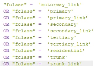
Double click on Fields and Values and select fclass
Click on the “=” operator on the bottom left of the expression box
Click on All Unique and scroll down to select motorway
Manually type in OR and repeat steps 4-6 for motorway_link, primary, primary_link, secondary, secondary_link, tertiary, tertiary_link, residential, trunk and trunk_link
- Click on Select Features and close the dialog window
2.2.4.4 Exporting the selected motor vehicle network as GeoPackage
Right click on all_roads layer
Select Export > Save selected feature as
File type: GeoPackage
File Name: SG
- Select SG.gpkg that was previously created
Layer Name: SG – roads
Remove the all_roads layer from the Panel
* Note: The layer is now in SVY21 Projected Coordinate System and not in original WGS84 Geographic Coordinate System
Now that all the motor vehicle network within Singapore is extracted, we will move on to create a hexagon layer which would be used in QNEAT3 for the accessibility analysis
2.2.5 Creating Hexagon Layer using MasterPlan 14
From the menu bar, select Vector > Research Tools > Create Grid
Create Grids dialog window appears
Grid Type: Hexagon (Polygon) from drop down list
Grid Extend: Calculate from Layer > MasterPlan 14
Horizontal Spacing: 500
Vertical Spacing: 500
Grid CRS: EPSG 3414
When you are ready to run the process, click on Run
Reminder: Read the Log before closing the dialog window
Click on Close after the process is finished
* Notice that a new temporary layer called Grid is added onto the layer pane and display on Map window
2.2.5.1 Editing the Hexagon Layer
Select Vector > Geoprocessing Tools > Clip
Clip Dialog window appears
Input layer: Grid
Overlay layer: MasterPlan 14
Click on Advanced Options
- Invalid Feature Filtering: Do not Filter (Better Performance)
* Repeat this step for Overlay Layer
- Click Run and then Close to close the dialog window
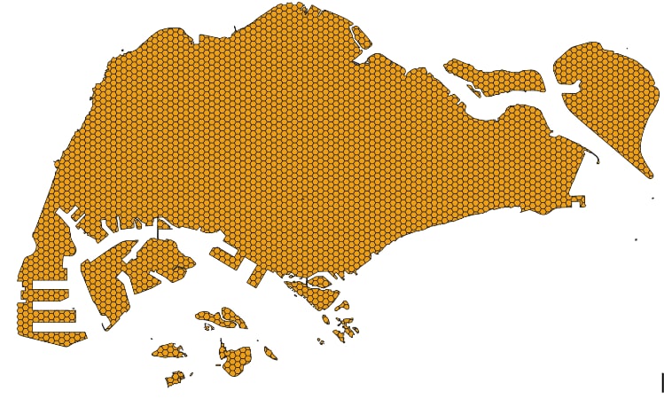
- Repeat the steps above to save Clipped virtual layer into GeoPackage and call the data layer as Hexagon
- Remove the Clipper virtual layer, Grid layers from the Layer Panel
Your screen should look something similar to this.
In general, network analysis required the demand in a point feature. Hexagon, on the other hand, is a polygon feature. As such, we would have to compute the centroids of the hexagon.
2.2.6 Computing Hexagon Centroid
From the menu bar, select Vector > Geometry Tools > Centroids
Centroids Dialog window appears
- Input Layer: Hexagon
Click on Run button
Reminder: Read the Log before closing the dialog window
Click on Close after the process is finished
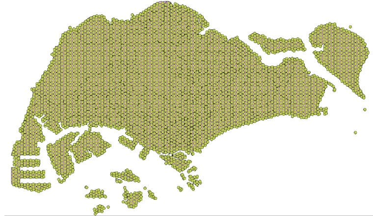
* Notice that a new temporary layer called Centroid is added onto the Layers panel and displayed on Map view.
Your screen should looks similar to this
2.2.6.1 Saving the Centroid Layer
Repeat the steps to export as GeoPackage and name the newly created layer as hex_centroid
Remember to remove the temporary centroids layer
2.3 Accessibility Analysis
This section, we will be performing network accessibility analysis by using QGIS Network Analysis Toolbox (QNEAT3) Plugin
2.3.1 Installing QNEAT3 Plugin
Select Plugins > Manage and Install Plugin
At the Plugin dialog window, type QNEAT3
Notice that QNEAT3 appears on the search output list
Click on QNEAT3 and Install Plugin button
When the installation is completed, close the dialog box by clicking on the Close button
2.3.2 Working with OD Matrix Tool
Origin-Destination Matrix (OD Matrix) tool of QNEAT3 plugin will be used to calculate the distance between hexagon centroid (as the demand points) and eldercare centres (as the supply points)
From the menu bar, click on Processing > Toolbox
At the Search pane, type OD Matrix
Click on OD Matrix Layers as Table (m:n).
OD Matrix Layers as Table (m:n) dialog window appears.
For Network Layer, select roads from the drop-down list.
For From-Point Layer, select hex_centroid from the drop-down list.
For Unique Point ID Field, select fid from the drop-down list.
For To-Point Layer, select MergedJC from the drop-down list.
For Unique Point ID Field, select fid from the drop-down list.
For Optimization Criterion, select Shortest Path (distance optimization) from the drop-down list.
For Entry Cost calculation method, select Ellipsoidal from the drop-down list.
For Direction field, select oneway from the drop-down list.
For Value for forward direction, type F.
For Value for backward direction, type T.
For Value for both direction, type B.
For Topology tolerance, type 0.5 (i.e. 0.5 m).
When you are ready, click on Close to close the dialog window
* Notice that new temporary table called Output OD Matrix is added onto Layers panel
At the Layers panel, right-click on Output OD Matrix and select Open Attribute Table from the context menu
Using the steps to export into GeoPackage, save the temporary Output OD Matrix table as GeoPackage format. Name the layer OD_mixedjc
2.3.3 Extracting Shortest Distance Pairs
Next, use the SQL tool of QGIS to select destination points with the shortest distance.
At the Search pane of Processing Toolbox, type SQL
Double-click on Execute SQL of Vector general.
Execute SQL dialog window appears.
For Additional input datasources, select on the button at the right end.
Click on the checkbox Output OD Matrix.
Click on OK button.
At SQL query panel, type the following SQL
- Select origin_id, destination_id, min(total_cost) as shortest_distance from input1 group by origin_id
For Geometry type, select No Geometry from the drop-down list
* Notice that a temporary table called SQL Output is added onto Layers panel. It consists of four fields. The values in shortest_distance field are shortest distance between demand points and its nearest Junior Colleges
- Using the steps to export into GeoPackage, save the temporary SQL Output as GeoPackage format. Name the layer acc_mixedjc
2.3.4 Mapping Accessibility Values
Use the mapping function of QGIS to show the distribution of accessibility to Junior College
2.3.4.1 Creating a Duplicate layer
At the Layers panel, right-click on the hexagon layer and select Duplicate Layer from the context menu.
A new layer called hexagon copy is added onto the Layers panel.
Rename the layer to Accessibility to mixedjc
2.3.4.2 Performing Relational Join
Before we can prepare the choropleth map, we need to join acc_mixedjc data table to the newly created Accessibility to mixedjc by using fid of acc_mixedjc data table and fid of Accessibility to mixedjc attribute table as unique join fields.
At the Layer panel, right-click on Accessibility to mixedjc layer and select Properties from the context menu.
The Properties dialog window appears.
At the option panel, click on Joins.
Click on + button to add a join.
The Add Vector Join dialog window appears.
For the Join layer, select acc_mixedjc from th drop-down list.
For the Join field, select fid from the drop-down list.
For the Target field, select fid from the drop-down list.
Keep the checkbox in front of the Cache join layer in memory checked.
When one, click on OK button
2.3.4.3 Preparing Choropleth Map
Double click on Accessibility to mixedjc
Layer Properties dialog windows appears
Click on Symbology
At Symbol selection drop-down list, select Graduated from the drop-down list
Value: SG — acc_mixedjc_shortest_distance
Classes – keep it as 5
Colour Ramp – any colour of your choice
Mode: Natural Break (Jenks) from the drop-down list
Click on Classify
Click on Histogram > Load Values
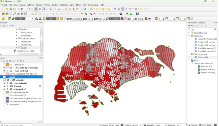
Click on Apply
The choropleth map should like something like this.
2.4 Repeat of steps for schools before the merger
- 2.2.3, 2.2.5, 2.2.6 and 2.3 to produce another choropleth map
2.5 Public Transports near Junior Colleges
2.5.1 Creating buffer region
Select Vector > Geoprocessing Tools > Buffer…
Buffer Dialog Window
Input Layer: SG – Merged JC
Distance: 1000
Segments: 100
check the Dissolve results
Click on Run
Click on Close
Notice that a new GIS layer called Buffered has been added to the Browser panel
Save the output buffering layer into GeoPackage format. Name the newly created layer dissolved
2.5.2 Identifying bus stops within the buffer region
2.5.2.1 Filtering bus stops
Click on Layer >Add Vector Layer
Click on “...”
Select the downloaded gis_osm_transport_a_free_1 from Subtheme1 folder
Select attribute table
Click on Select By Expression and a dialog window will appear
Double click on Fields and Values and select fclass
Click on the “=” operator on the bottom left of the expression box
Click on All Unique and scroll down to select bus
Click on Select Features and close the dialog window
2.5.2.2 Saving bus stops layer as GeoPackage
Right click on gis_osm_transport_a_free_1 layer
Select Export > Save selected feature as
File type: GeoPackage
File Name: SG
Select SG.gpkg that was previously created
Layer Name: SG – BUS STOPS
Remove the gis_osm_transport_a_free_1 layer from the Panel
2.5.2.3 Identifying bus stops within buffer region
Select Vector > Geoprocessing Tools > Clip
Clip Dialog window appears
Input layer: dissolved
Overlay layer: SG – BUS STOPS
Click on Advanced Options
Invalid Feature Filtering: Do not Filter (Better Performance)
Click Run and then Close to close the dialog window
Repeat the steps above to save Clipped virtual layer into GeoPackage and call the data layer as SG – bus within buffer
Remove the Clipper virtual layer from the Layer Panel
2.5.3 Identifying MRT stations within buffer region
2.5.3.1 Importing MRT and LRT data
Click on Layer >Add Vector Layer
Click on “...”
Select the downloaded lta-mrt-station-exit from Subtheme1 folder
Remove extra fields and only keep “fid”, “STATION_NA” and “EXIT_CODE”
Save the layer as GeoPackage and call the data layer SG – MRT STATIONS
2.5.3.2 Identifying MRT and LRT stations within buffer region
Select Vector > Geoprocessing Tools > Clip
Clip Dialog window appears
Input layer: dissolved
Overlay layer: SG – MRT STATIONS
Click on Advanced Options
Invalid Feature Filtering: Do not Filter (Better Performance)
Click Run and then Close to close the dialog window
Repeat the steps above to save Clipped virtual layer into GeoPackage and call the data layer as SG – mrt within buffer
Remove the Clipper virtual layer from the Layer Panel
2.6 Repeat of steps for schools before the merger
- Repeat steps 2.5.1, 2.5.2.3, 2.5.3.2 in sequence, while using the locations of Junior Colleges to create a new 1 km buffer region